How does Network Toolkit calculate potentials ?

There are a number of methods of calculating retail and service potentials. All of them involve ‘allocating’ potential from the residential postcodes, zipcodes or geography where the potential resides to the dealer network. In order to explain this, it is important to understand that there is a common starting point for all of these methods; Before we can calculate potentials for the dealers, we must first have the potential available across the country at some level of geography.

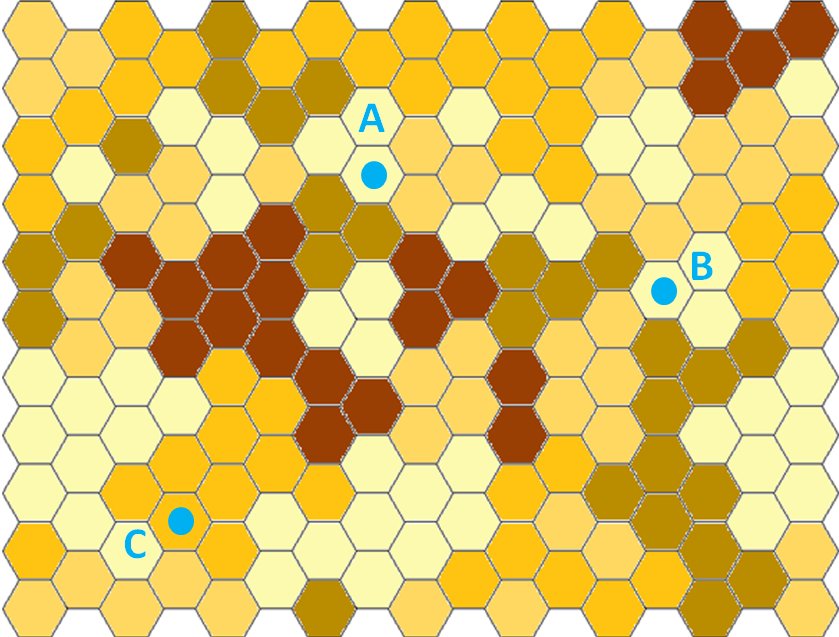
This is illustrated below in figure 1. The hexagon shapes represent some type of geography, such as postcode sectors (UK), Germeinde (Germany) or Communes (France). In each piece of geography, there is a demand (potential) for the product, usually expressed as an annual expected number of sales or annual demand for service. In our case, the level of demand is related to the shading; light yellow – small demand, dark brown – high demand. The Blue dots are the locations of dealers A, B and C. In this simple example, we should assume that this area represents the country, and that there are 3 dealers in the network.

Figure 1. Simple view of a dealer network showing potential by geography

We would assume that all of the potential sales or service for this brand, (shaded above) is going to be allocated to the 3 dealers (in blue) on the map.

There are 3 methods of calculating this potential in Network Toolkit and these are explained below. For each method, the extent of any drivetime is represented by the blue circles or shapes.

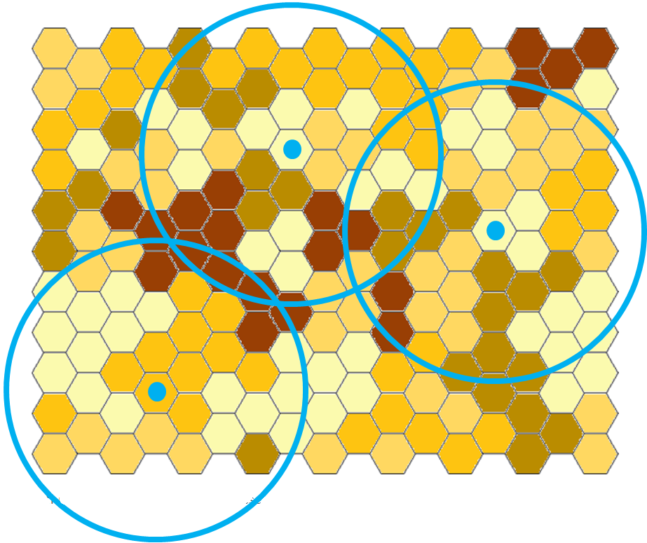
1. Simple drivedistance / drivetime

The most simple method simply calculates a drivetime of x minutes from each dealer. All potential within this drivetime is allocated to the dealer. Since a drivetime from one dealer may overlap with another, there is often ‘double counting’ so that potential allocated to one dealer is also allocated to another dealer. If we added up the overall potential allocated to all dealers in the country, the figure would be greater than the total available potential in the country.

Figure 2. Simple drivedistance

In this example, the blue circles represent a 30 minute drivetime from each dealer.

Pros:

Simple to understand

Good for comparing what lies within x minutes of a dealer

Cons:

Can’t calculate impact upon like brand dealers

Overlapping and double counting of potentials

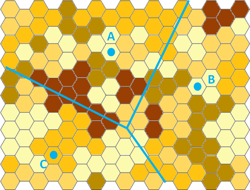
2. Equidistance

Figure 3. Equidistance method

With this method, each piece of geography (and it’s potential) is allocated to the nearest dealer on a drivetime or drivedistance basis. The method is fairly realistic because it models customer behaviour to the extent that drivetime or drivedistance is a key part of their consideration in choosing where to buy, although no other factors are taken into consideration. The impact on surrounding dealers can also be calculated.

Pros:

Fairly realistic as it takes drivetime, drivedistance into account

Simple concept to understand / easy to calculate

Impact calculated on surrounding dealers

Cons:

Only drivetime is used

Assumes that all the potential from one location will go to a single dealer

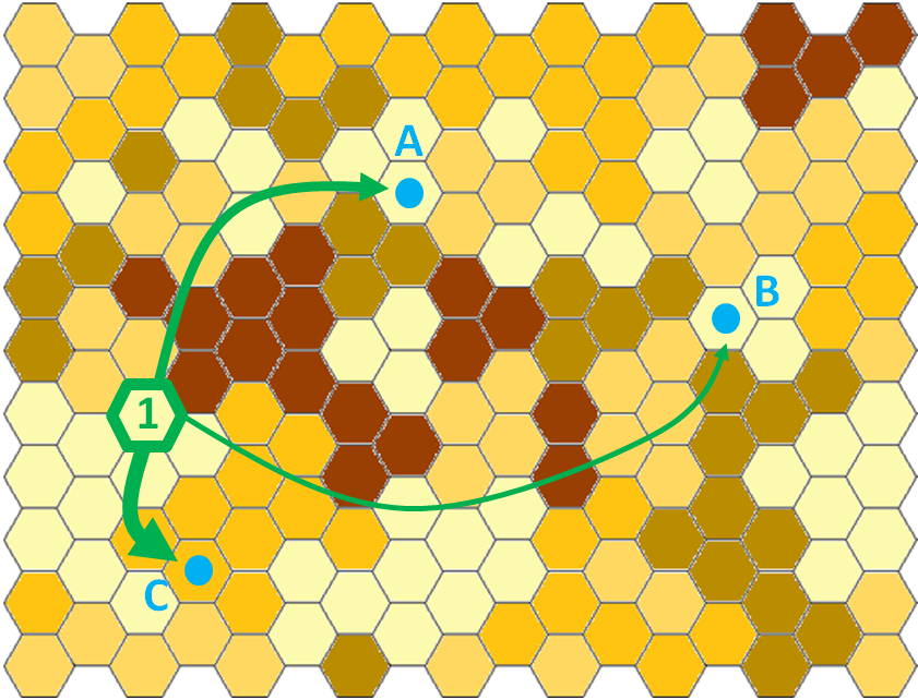
3. SIM (Gravity Model or Spatial Interaction model)

The gravity model is the most sophisticated and accurate method of allocation potential to dealers. It uses 3 main factors to determine where customers will shop and models customer behaviour more accurately than any other method.

Figure 4. Gravity model – calculating the allocation from one of many geography polygons

The potential in each piece of geography is allocated to several dealers, based upon the relative drivetime or drivedistance from that location to each dealer. In this example, assume that the potential at location 1 is 100 units. These units will be split between dealers A, B and C based upon the drivetime or distance, so most units would be allocated to dealer C, followed by dealer A and then B (illustrated by the thickness of the green arrows). In addition, two other factors are used to determine this split.

The ‘attractiveness’ or ‘pull’ (hence the name gravity model) of the dealers is independently calculated, based upon size, facilities, landtype( metropolitan v’s rural) and whether they are close to dealers of competitor brands. The various ‘attractiveness’ scores of each dealer will ‘pull’ on the potential to varying degrees, adjusting the initial splits calculated from drivetime alone.

Finally, intervening opportunities will decrease or increase the potential within each piece of geography. If there are many dealers of competing brands close to one location but no dealers from your own brand, the actual potential in that location will decrease. The opposite will also happen.

Competition is a ‘double-edged’ sword here; It increases the ‘attractiveness’ or pull of a dealer location, but it also increases the competition or choice to the customer. It’s rather like increasing the size of the pie, but providing you with a smaller slice.

Pros:

Most accurate and realistic method of modelling customer behaviour

Full impact on dealers and for the brand nationally

Cons:

A ‘black box’ method, complicated to explain and difficult to clarify

Requires more detailed datasets